

By Kamil Jankowski | Business Intelligence Engineer
Survival Analysis uses statistical methods and time-to-event variables to predict that a patient, device, or other objects of interest will survive past a specific time. Its original use is well known in healthcare and life insurance since survival analysis can estimate mortality rates from illness and disease. However, today’s businesses leverage this technique in sectors like finance, manufacturing, or services to calculate events such as bankruptcy, electronic devices’ lifecycle, or customer churn.
In this article, I will present a survival analysis on the example of fictional users to calculate their probability of surviving after X months since the registration date, compare the survival rates for two groups of users, and estimate the lifetime value for the company. If you are interested in business analysis, I encourage you to read, as well, an article about Custom Email Reports.
How Does Survival Analysis Work – Survival Function
The core of Survival Analysis is a mathematical function called “survival” which the following formula can represent:

The quantity T refers to specific time characteristics of an individual object of interest. For instance, the variable T may refer to the age at which the object of interest stopped working. In this case, survival function S(t) can be interpreted as the probability that an object of interest is still working after age t. If S(5) = 0.75, it means that 75% of the objects of interest in the population should still be working at the age of 5 (will survive pastime t = 5).
To demonstrate the Survival Analysis, I decided to use the lifelines Python library (not a built-in one, but available to be installed).
What Is The Probability That Users Will Churn – Kaplan-Meier Estimator And Survival Curve
Test data set loaded into Python include columns: user_id, weeks_active (date difference between the week of user registration and the week of analysis), is_still_active (boolean variable where 0 represents the user has churned while 1 that the user is still active), and premium_user (boolean variable where 0 represents regular users and 1 represents users who paid for optional subscription). It is worth mentioning that our premium_user could be used to prepare other user cohorts, e.g. users who registered using referral links or users who are using different OS versions (e.g. Android vs iOS users). The additional cohort can be used to test the hypothesis that users in cohort B have a lower rate than users in cohort A.
| user_id | weeks_active | is_still_active | premium_user |
| 1 | 35 | 1 | 0 |
| 2 | 17 | 0 | 1 |
| 3 | 4 | 0 | 0 |
| 4 | 21 | 1 | 1 |
Once the data set is loaded, we can use the Kaplan-Meier estimator, which is one of the most popular and easiest-to-use methods in Survival Analysis that estimates the survival function. We need to fit the model by selecting a duration and events observed.
from lifelines import KaplanMeierFitter
kmf = KaplanMeierFitter()
kmf.fit(durations=df['weeks_active'],
event_observed=df['is_still_active'])
In this particular dataset, we can observe 2824 right-censored observations among 15531 total observations. Normally, datasets usually contain censoring since we use time-to-event data. That is why, for some objects of interest, it is not possible to capture their survival time. There are three types of censoring: right, left, and interval. Right censoring means that the true survival time of an object is greater than the recorded survival time, while left censoring is the opposite. Interval censoring happens when the true survival time lies within a certain range.
Now the model is ready to visualize the results on the Kaplan-Meier plot. To do that, we can use the matplotlib package.
import matplotlib.pyplot as plt
kmf.plot(ci_show=False)
plt.ylabel('Survival Rate')
plt.title('Survival Curve')
plt.show()

As can be easily seen, the Survival Rate decreases with time and after almost a year since the registration, only around 10% of users are still active. In the example below, it is shown how to predict an accurate Survival Rate after a given time period:
survival_12 = kmf.predict(12)*100
print(f'Survival rate after 12 weeks: {round(survival_12,2)}%')
In our case, the Survival Rate for 12 weeks is 29% which means that 29% of regular users will not churn after 12 weeks from registration week.
Does Churn Probability Lower For Premium Users Than For Regular Ones?
Survival Analysis can also be used for comparing the churn ratios between two or more user cohorts. I decided to check if users who are paying for some premium functionalities such as ads-free or unlimited song skipping have a lower churn rate than users who are not paying for that. Before we will test our hypothesis, we need to subset data for each group of users and fit the Kaplan-Meier estimator for each of them.
# creating subsets for each group
df_fin = df[df['premium_user']==1]
df_no_fin = df[df['premium_user']==0]

# plotting survival curve for premium users
kmf_fin = KaplanMeierFitter()
kmf_fin.fit(df['weeks_active'], df_fin['is_still_active'], label='Premium Users')
ax = kmf_fin.plot(ci_show=False)

# plotting survival curve for regular users
kmf_no_fin = KaplanMeierFitter()
kmf_no_fin.fit(df['weeks_active'], df_no_fin['is_still_active'], label='Regular Users')
ax = kmf_no_fin.plot(ci_show=False)

# labels
plt.ylabel('Survival Rate')
plt.title('Survival Curve')
plt.show()
Using the matplotlib plot, we can again visualize the results on the line chart.
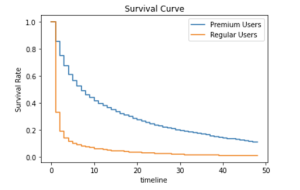
The difference between both cohorts is easy to notice, but is it statistically significant? We can (and we should) check it with a log-rank test, which is a nonparametric test used when the data is right-censored. In a nutshell, this hypothesis test compares the survival distributions of two samples. But before we start testing the dataset, we need to define our null and alternative hypotheses.
H0 – Premium Users have a similar Survival Rate to Regular Users
H1 – Premium Users have a different Survival Rate than Regular Users
from lifelines.statistics import logrank_test
# perform log rank test
results = logrank_test(durations_A=df_fin['weeks_active'],
                      event_observed_A=df_fin['premium_user'],
                      durations_B=df_no_fin['weeks_active'],
                      event_observed_B=df_no_fin['premium_user'])

results = results.summary
print(f'P-value: {results.p[0]}')
For our dataset, the returned p-value is much lower than 1% which means that we can reject the null hypothesis, so Survival Rate for Premium Users is statistically significant, and these users have a higher rate than Regular ones.
Summary
As shown in this article, Survival Analysis can be easily utilized for a better understanding of churn. Moreover, the same script can also be used for calculating device lifecycle or bankruptcy forecasting. To learn more about it, I recommend starting with the following articles and tutorials:
- https://towardsdatascience.com/what-is-survival-analysis-examples-by-hand-and-in-r-3f0870c3203f
- https://www.graphpad.com/guides/survival-analysis
- http://www.biecek.pl/statystykaMedyczna/Stevenson_survival_analysis_195.721.pdf
We can’t stress enough that Survival Analysis helps organizations make informed decisions about their customer base, allowing them to identify and address potential issues before they become serious. At CRODU we provide expert advice on custom software development and business-related tools for a wide range of industries. For further advice, contact us here.